Kurtosis

Computes the kurtosis, $\gamma_{2}$, of the values in x with optional adjustment to give $G_{2}$, the expected populaton value of kurtosis from a sample.

Usage

kurtosis(x, xs = TRUE, adjust = TRUE)

Arguments

x: a numeric vector.
xs: logical, indicating whether to calculate excess kurtosis i.e., the difference from the kurtosis of the normal distribution; default TRUE.
adjust: logical, indicating whether x is a sample from a population; default TRUE.

Value

A numeric containing the kurtosis value.

Details

Moments for samples of size n are given by: -

$$m_{r} = \displaystyle \frac{\sum \left(x - \overline{x} \right)^{r}}{n}$$

The (excess) kurtosis $\gamma_{2}$ of a numeric variable is the fourth moment ($m_{4}$) about the mean rendered dimensionless by dividing by the square of the second moment ($m_{2}$), from which 3, the value of ($m_{4}/m_{2}^2$) for the normal distribution is subtracted: -

$$\gamma_{2} = \displaystyle \frac{m_4}{{m_{2}}^2} - 3$$

The expected population value of (excess) kurtosis $G_{2}$ from a sample is obtained using: -

$$G_{2} = \displaystyle \frac{(n - 1)}{(n-2)(n-3)}[(n+1)\gamma_{2} + 6]$$

(Adapted from Crawley, 2012, and Joanes and Gill, 1998.)

References

Crawley, Michael J. (2012) The R Book. John Wiley & Sons, Incorporated. ISBN:9780470973929. p.350-352. doi:10.1002/9781118448908

Joanes, D.N., and Gill, C.A. (1998). Comparing measures of sample kurtosis and kurtosis. Journal of the Royal Statistical Society. Series D (The Statistician) 47(1): 183–189. doi:10.1111/1467-9884.00122

Examples

 ## Heights of 100 randomly selected male university students, adapted from Spiegel and Stephens
 ## (Theory and Problems of Statistics. 4th edn. McGraw-Hill. 1999. ISBN 9780071755498).
 table(heights)
#> heights
#> 61 64 67 70 73 
#>  5 18 42 27  8 
 hist(heights, seq(59.5, 74.5, 3))

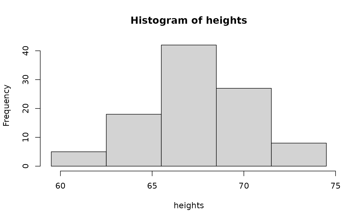 kurtosis(heights) 
#> [1] -0.2091471
 kurtosis(heights, adjust = FALSE)
#> [1] -0.258241

 ## Litter sizes in albino rats (n = 815), data from King (1924; Litter production and
 ## the sex ratio in various strains of rats. The Anatomical Record 27(5), 337-366).
 table(litter_sizes)
#> litter_sizes
#>   1   2   3   4   5   6   7   8   9  10  11  12 
#>   7  33  58 116 125 126 121 107  56  37  25   4 
 hist(litter_sizes, 0:12)

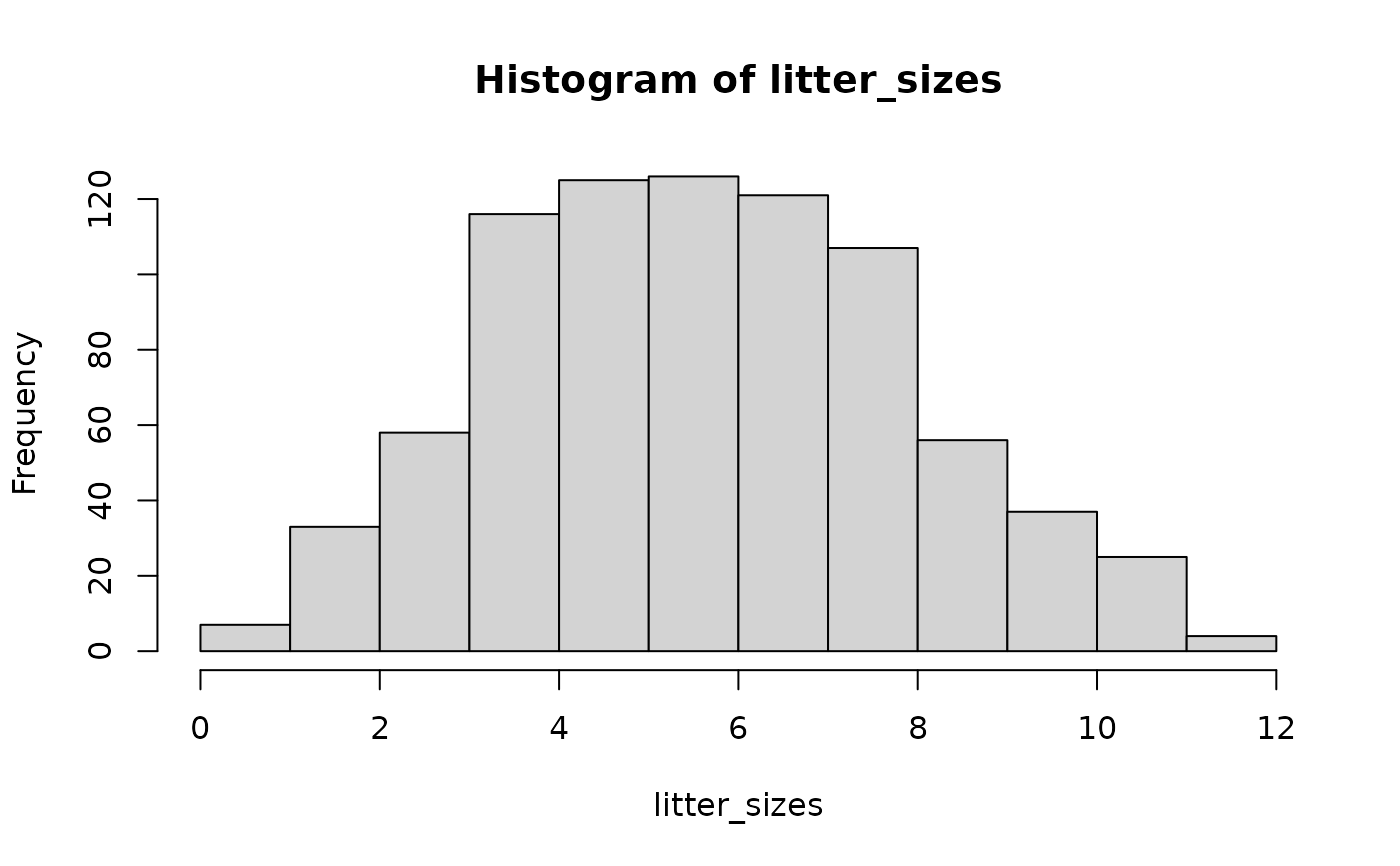 kurtosis(litter_sizes) 
#> [1] -0.4761573
 kurtosis(litter_sizes, adjust = FALSE)
#> [1] -0.4805941